Chapter 8 Data Wrangling with dplyr and tidyr
The package dplyr is an R package for making tabular data wrangling easier by using a limited set of functions that can be combined to extract and summarize insights from your data. It pairs nicely with the package tidyr, enabling you to swiftly convert between different data formats (long vs. wide) for plotting and analysis.
dplyr is built to work directly with dataframes, with many common tasks optimized by being written in a compiled language (C++) (not all R packages are written in R!).
The package tidyr addresses the common problem of reshaping your data for plotting and use by different R functions. Sometimes we want data sets where we have one row per measurement. Sometimes we want a dataframe where each measurement type has its own column, and rows are instead more aggregated groups. Moving back and forth between these formats is nontrivial, and tidyr gives you tools for this and more sophisticated data wrangling.
8.1 Learning dplyr
Below we will work on COVID-19 county level infected count data, and we can obtain the data from Github R package slid.
# Install the slid package from github
# library(devtools)
# devtools::install_github('covid19-dashboard-us/slid')
# Load objects in I.county into my workspace
library(slid)
data(I.county)

# preview the data
# View(I.county)
We’re going to learn some of the most common dplyr functions:
select(): subset columnsfilter(): subset rows on conditionsmutate(): create new columns by using information from other columnsgroup_by()andsummarize(): create summary statistics on grouped dataarrange(): sort resultscount(): count discrete values
8.2 Selecting columns and filtering rows
- To select columns of a dataframe, use
select(). The first argument to this function is the dataframe (I.county), and the subsequent arguments are the columns to keep, separated by commas. Alternatively, if you are selecting columns adjacent to each other, you can use a:to select a range of columns, read as “select columns from __ to __.”
# load the tidyverse
dplyr::select(I.county, ID, County, State)
# to select a series of connected columns
dplyr::select(I.county, ID, County, State,
X2020.12.11:X2020.12.01)- To choose rows based on specific criteria, we can use the
filter()function. The arguments after the dataframe are the condition(s) we want for our final dataframe to adhere to (e.g.Statename is “Iowa”). We can chain a series of conditions together using commas between each condition.
- Here is an example of
filter()function with multiple conditions:
# multiple conditions: all Iowa counties with cumulative
# infection count > 10000
dplyr::filter(I.county, State == "Iowa",
              X2020.12.11 > 10000)
Figure 8.1 shows some commonly used R logic omparisons
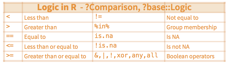
Figure 8.1: Some commonly used logic comparisons.
8.3 Pipes
What if you want to select and filter at the same time? There are three ways to do this: use intermediate steps, nested functions, or pipes.
With intermediate steps, you create a temporary dataframe and use that as input to the next function, like this:
Iowa.I.county <-
  dplyr::filter(I.county, State == "Iowa")
Iowa.I.county.DEC <-
  dplyr::select(Iowa.I.county, X2020.12.11:X2020.12.01)
This is readable, but can clutter up your workspace with lots of objects that you have to name individually. With multiple steps, that can be hard to keep track of.
You can also nest functions (i.e. one function inside of another), like this:
Iowa.I.county.DEC <-
  dplyr::select(dplyr::filter(I.county, State == "Iowa"),
                ID, County, State, X2020.12.11:X2020.12.01)
This is handy but can be difficult to read if too many functions are nested, as R evaluates the expression from the inside out (in this case, filtering, then selecting).
The last option, pipes, are a recent addition to R. Pipes let you take the output of one function and send it directly to the next, which is useful when you need to do many things to the same dataset. Pipes in R look like %>% and are made available via the magrittr package, installed automatically with dplyr.
In the above code, we use the pipe to send the interviews dataset first through filter() to keep rows for the state of Iowa, then through select() to keep only the count in December. Since %>% takes the object on its left and passes it as the first argument to the function on its right, we don’t need to explicitly include the dataframe as an argument to the filter() and select() functions anymore.
Some may find it helpful to read the pipe like the word “then”. For instance, in the above example, we take the dataframe I.county, then we filter for rows with State == "Iowa", then we select columns from X2020.12.11 to X2020.12.01. The dplyr functions are somewhat simple, but by combining them into linear workflows with the pipe, we can accomplish more complex data wrangling operations.
If we want to create a new object with this smaller version of the data, we can assign it a new name:
Iowa.I.county.DEC <- I.county %>%
  dplyr::filter(State == "Iowa") %>%
    dplyr::select(ID, County, X2020.12.11:X2020.12.01)

head(Iowa.I.county.DEC)
## ID County X2020.12.11 X2020.12.10 X2020.12.09
## 1 19001 Adair 506 503 499
## 2 19003 Adams 208 206 200
## 3 19005 Allamakee 995 990 971
## 4 19007 Appanoose 868 862 858
## 5 19009 Audubon 326 323 321
## 6 19011 Benton 1852 1847 1826
## X2020.12.08 X2020.12.07 X2020.12.06 X2020.12.05
## 1 489 484 484 479
## 2 196 196 195 193
## 3 954 939 925 922
## 4 853 849 843 839
## 5 315 314 313 312
## 6 1819 1798 1789 1778
## X2020.12.04 X2020.12.03 X2020.12.02 X2020.12.01
## 1 472 453 448 444
## 2 188 181 179 171
## 3 912 884 870 850
## 4 834 816 807 804
## 5 312 311 305 301
## 6 1769 1754 1740 17288.4 Select and order top n entries (by group if grouped data).
The function top_n can be used to select top (or bottom) n rows (by value).
This is a convenient wrapper that uses filter()and min_rank() to select the top or bottom entries in each group, ordered by wt.
** Usage **
** Arguments **
* x: a tbl() to filter
* n: number of rows to return. If x is grouped, this is the number of rows per group. Will include more than n rows if there are ties. If n is positive, selects the top n rows. If negative, selects the bottom n rows.
* wt (Optional). The variable to use for ordering. If not specified, defaults to the last variable in the tbl.
This argument is automatically quoted and later evaluated in the context of the data frame. It supports unquoting.
Let us find the top ten counties with the largest cumulative infected count on December 11, 2020.
##  [1] Maricopa      LosAngeles    SanBernardino Broward
##  [5] Miami-Dade    Cook          Clark         Dallas
##  [9] Harris        Tarrant
## 1839 Levels: Abbeville AcadiaParish Accomack Ada ... obrien
Let us find the top ten counties with the smallest cumulative infected count on December 11, 2020.
library(dplyr)
I.county.bottom10 <- I.county %>%
  top_n(-10, wt = X2020.12.11)
I.county.bottom10$County
## [1] Dukes Nantucket OglalaLakota Beaver
## [5] BoxElder Cache Carbon Daggett
## [9] Duchesne Emery Garfield Grand
## [13] Iron Juab Kane Millard
## [17] Morgan Piute Rich Sanpete
## [21] Sevier Uintah Washington Wayne
## [25] Weber
## 1839 Levels: Abbeville AcadiaParish Accomack Ada ... obrienLet us find the county with the largest cumulative infected count on December 11, 2020 for each state.
8.5 Mutate
Frequently you’ll want to create new columns based on the values in existing columns, for example, to obtain the number of daily new cases based on the cumulative count. For this, we’ll use mutate().
I.county.new <- I.county %>%
    dplyr::filter(State == "Iowa") %>%
    dplyr::select(ID, County, X2020.12.11:X2020.12.10) %>%
    mutate(Y2020.12.11 = X2020.12.11 - X2020.12.10)

head(I.county.new)
## ID County X2020.12.11 X2020.12.10 Y2020.12.11
## 1 19001 Adair 506 503 3
## 2 19003 Adams 208 206 2
## 3 19005 Allamakee 995 990 5
## 4 19007 Appanoose 868 862 6
## 5 19009 Audubon 326 323 3
## 6 19011 Benton 1852 1847 5If we want to obtain the number of daily new cases based on the cumulative count for the dates in December only, we can try the following:
I.county.Iowa <- I.county %>%
  dplyr::filter(State == "Iowa")

I.county.tmp = I.county.Iowa[, -(1:3)]
I.county.Iowa.new = I.county.Iowa
I.county.Iowa.new[, -(1:3)] =
  I.county.tmp - cbind(I.county.tmp[, -1], 0)

I.county.Iowa.DEC = I.county.Iowa.new %>%
dplyr::select(ID, County, X2020.12.11:X2020.12.01)

name.tmp = substring(names(I.county.Iowa.DEC)[-(1:2)], 2)
names(I.county.Iowa.DEC)[-(1:2)] = paste0("Y", name.tmp)
head(I.county.Iowa.DEC)
## ID County Y2020.12.11 Y2020.12.10 Y2020.12.09
## 1 19001 Adair 3 4 10
## 2 19003 Adams 2 6 4
## 3 19005 Allamakee 5 19 17
## 4 19007 Appanoose 6 4 5
## 5 19009 Audubon 3 2 6
## 6 19011 Benton 5 21 7
## Y2020.12.08 Y2020.12.07 Y2020.12.06 Y2020.12.05
## 1 5 0 5 7
## 2 0 1 2 5
## 3 15 14 3 10
## 4 4 6 4 5
## 5 1 1 1 0
## 6 21 9 11 9
## Y2020.12.04 Y2020.12.03 Y2020.12.02 Y2020.12.01
## 1 19 5 4 3
## 2 7 2 8 0
## 3 28 14 20 22
## 4 18 9 3 5
## 5 1 6 4 1
## 6 15 14 12 108.6 Split-apply-combine data analysis and the summarize() function
Many data analysis tasks can be approached using the split-apply-combine paradigm: split the data into groups, apply some analysis to each group, and then combine the results. dplyr makes this very easy via the group_by() function.
The summarize() function
Summarize uses summary functions, functions that take a vector of values and return a single value, such as:
dplyr::first: First value of a vector.dplyr::last: Last value of a vector.dplyr::nth: Nth value of a vector.dplyr::n: # of values in a vector.dplyr::n_distinct: # of distinct values in a vector.IQR: IQR of a vector.min: Minimum value in a vector.max: Maximum value in a vector.mean: Mean value of a vector.median: Median value of a vector.var: Variance of a vector.sd: Standard deviation of a vector.
group_by() is often used together with summarize(), which collapses each group into a single-row summary of that group. group_by() takes as arguments the column names that contain the categorical variables for which you want to calculate the summary statistics. Once the data are grouped, you can also summarize multiple variables simultaneously (and not necessarily on the same variable). So to compute the state level infected count by State:
I.state <- I.county %>%
  group_by(State) %>%
  summarize(across(X2020.12.11:X2020.01.22,
                   ~ sum(.x, na.rm = TRUE)))
## `summarise()` ungrouping output (override with `.groups` argument)## # A tibble: 2 x 326
## State X2020.12.11 X2020.12.10 X2020.12.09 X2020.12.08
## <fct> <int> <int> <int> <int>
## 1 Alab… 288775 284922 280187 276665
## 2 Ariz… 394512 387529 382601 378157
## # … with 321 more variables: X2020.12.07 <int>,
## # X2020.12.06 <int>, X2020.12.05 <int>,
## # X2020.12.04 <int>, X2020.12.03 <int>,
## # X2020.12.02 <int>, X2020.12.01 <int>,
## # X2020.11.30 <int>, X2020.11.29 <int>,
## # X2020.11.28 <int>, X2020.11.27 <int>,
## # X2020.11.26 <int>, X2020.11.25 <int>,
## # X2020.11.24 <int>, X2020.11.23 <int>,
## # X2020.11.22 <int>, X2020.11.21 <int>,
## # X2020.11.20 <int>, X2020.11.19 <int>,
## # X2020.11.18 <int>, X2020.11.17 <int>,
## # X2020.11.16 <int>, X2020.11.15 <int>,
## # X2020.11.14 <int>, X2020.11.13 <int>,
## # X2020.11.12 <int>, X2020.11.11 <int>,
## # X2020.11.10 <int>, X2020.11.09 <int>,
## # X2020.11.08 <int>, X2020.11.07 <int>,
## # X2020.11.06 <int>, X2020.11.05 <int>,
## # X2020.11.04 <int>, X2020.11.03 <int>,
## # X2020.11.02 <int>, X2020.11.01 <int>,
## # X2020.10.31 <int>, X2020.10.30 <int>,
## # X2020.10.29 <int>, X2020.10.28 <int>,
## # X2020.10.27 <int>, X2020.10.26 <int>,
## # X2020.10.25 <int>, X2020.10.24 <int>,
## # X2020.10.23 <int>, X2020.10.22 <int>,
## # X2020.10.21 <int>, X2020.10.20 <int>,
## # X2020.10.19 <int>, X2020.10.18 <int>,
## # X2020.10.17 <int>, X2020.10.16 <int>,
## # X2020.10.15 <int>, X2020.10.14 <int>,
## # X2020.10.13 <int>, X2020.10.12 <int>,
## # X2020.10.11 <int>, X2020.10.10 <int>,
## # X2020.10.09 <int>, X2020.10.08 <int>,
## # X2020.10.07 <int>, X2020.10.06 <int>,
## # X2020.10.05 <int>, X2020.10.04 <int>,
## # X2020.10.03 <int>, X2020.10.02 <int>,
## # X2020.10.01 <int>, X2020.09.30 <int>,
## # X2020.09.29 <int>, X2020.09.28 <int>,
## # X2020.09.27 <int>, X2020.09.26 <int>,
## # X2020.09.25 <int>, X2020.09.24 <int>,
## # X2020.09.23 <int>, X2020.09.22 <int>,
## # X2020.09.21 <int>, X2020.09.20 <int>,
## # X2020.09.19 <int>, X2020.09.18 <int>,
## # X2020.09.17 <int>, X2020.09.16 <int>,
## # X2020.09.15 <int>, X2020.09.14 <int>,
## # X2020.09.13 <int>, X2020.09.12 <int>,
## # X2020.09.11 <int>, X2020.09.10 <int>,
## # X2020.09.09 <int>, X2020.09.08 <int>,
## # X2020.09.07 <int>, X2020.09.06 <int>,
## # X2020.09.05 <int>, X2020.09.04 <int>,
## # X2020.09.03 <int>, X2020.09.02 <int>,
## # X2020.09.01 <int>, X2020.08.31 <int>,
## # X2020.08.30 <int>, …or we can use summarise_at(), which affects variables selected with a character vector or vars():
I.state <- I.county %>%
  group_by(State) %>%
  summarize_at(vars(X2020.12.11:X2020.01.22),
               ~ sum(.x, na.rm = TRUE))

head(I.state, 2)
## # A tibble: 2 x 326
## State X2020.12.11 X2020.12.10 X2020.12.09 X2020.12.08
## <fct> <int> <int> <int> <int>
## 1 Alab… 288775 284922 280187 276665
## 2 Ariz… 394512 387529 382601 378157
## # … with 321 more variables: X2020.12.07 <int>,
## # X2020.12.06 <int>, X2020.12.05 <int>,
## # X2020.12.04 <int>, X2020.12.03 <int>,
## # X2020.12.02 <int>, X2020.12.01 <int>,
## # X2020.11.30 <int>, X2020.11.29 <int>,
## # X2020.11.28 <int>, X2020.11.27 <int>,
## # X2020.11.26 <int>, X2020.11.25 <int>,
## # X2020.11.24 <int>, X2020.11.23 <int>,
## # X2020.11.22 <int>, X2020.11.21 <int>,
## # X2020.11.20 <int>, X2020.11.19 <int>,
## # X2020.11.18 <int>, X2020.11.17 <int>,
## # X2020.11.16 <int>, X2020.11.15 <int>,
## # X2020.11.14 <int>, X2020.11.13 <int>,
## # X2020.11.12 <int>, X2020.11.11 <int>,
## # X2020.11.10 <int>, X2020.11.09 <int>,
## # X2020.11.08 <int>, X2020.11.07 <int>,
## # X2020.11.06 <int>, X2020.11.05 <int>,
## # X2020.11.04 <int>, X2020.11.03 <int>,
## # X2020.11.02 <int>, X2020.11.01 <int>,
## # X2020.10.31 <int>, X2020.10.30 <int>,
## # X2020.10.29 <int>, X2020.10.28 <int>,
## # X2020.10.27 <int>, X2020.10.26 <int>,
## # X2020.10.25 <int>, X2020.10.24 <int>,
## # X2020.10.23 <int>, X2020.10.22 <int>,
## # X2020.10.21 <int>, X2020.10.20 <int>,
## # X2020.10.19 <int>, X2020.10.18 <int>,
## # X2020.10.17 <int>, X2020.10.16 <int>,
## # X2020.10.15 <int>, X2020.10.14 <int>,
## # X2020.10.13 <int>, X2020.10.12 <int>,
## # X2020.10.11 <int>, X2020.10.10 <int>,
## # X2020.10.09 <int>, X2020.10.08 <int>,
## # X2020.10.07 <int>, X2020.10.06 <int>,
## # X2020.10.05 <int>, X2020.10.04 <int>,
## # X2020.10.03 <int>, X2020.10.02 <int>,
## # X2020.10.01 <int>, X2020.09.30 <int>,
## # X2020.09.29 <int>, X2020.09.28 <int>,
## # X2020.09.27 <int>, X2020.09.26 <int>,
## # X2020.09.25 <int>, X2020.09.24 <int>,
## # X2020.09.23 <int>, X2020.09.22 <int>,
## # X2020.09.21 <int>, X2020.09.20 <int>,
## # X2020.09.19 <int>, X2020.09.18 <int>,
## # X2020.09.17 <int>, X2020.09.16 <int>,
## # X2020.09.15 <int>, X2020.09.14 <int>,
## # X2020.09.13 <int>, X2020.09.12 <int>,
## # X2020.09.11 <int>, X2020.09.10 <int>,
## # X2020.09.09 <int>, X2020.09.08 <int>,
## # X2020.09.07 <int>, X2020.09.06 <int>,
## # X2020.09.05 <int>, X2020.09.04 <int>,
## # X2020.09.03 <int>, X2020.09.02 <int>,
## # X2020.09.01 <int>, X2020.08.31 <int>,
## # X2020.08.30 <int>, …or we can use summarise_if(), which affects variables selected with a predicate function:
I.state <- I.county %>%
  group_by(State) %>%
  summarize_if(is.numeric, ~ sum(.x, na.rm = TRUE))

head(I.state, 2)
## # A tibble: 2 x 327
## State ID X2020.12.11 X2020.12.10 X2020.12.09
## <fct> <int> <int> <int> <int>
## 1 Alab… 71489 288775 284922 280187
## 2 Ariz… 60208 394512 387529 382601
## # … with 322 more variables: X2020.12.08 <int>,
## # X2020.12.07 <int>, X2020.12.06 <int>,
## # X2020.12.05 <int>, X2020.12.04 <int>,
## # X2020.12.03 <int>, X2020.12.02 <int>,
## # X2020.12.01 <int>, X2020.11.30 <int>,
## # X2020.11.29 <int>, X2020.11.28 <int>,
## # X2020.11.27 <int>, X2020.11.26 <int>,
## # X2020.11.25 <int>, X2020.11.24 <int>,
## # X2020.11.23 <int>, X2020.11.22 <int>,
## # X2020.11.21 <int>, X2020.11.20 <int>,
## # X2020.11.19 <int>, X2020.11.18 <int>,
## # X2020.11.17 <int>, X2020.11.16 <int>,
## # X2020.11.15 <int>, X2020.11.14 <int>,
## # X2020.11.13 <int>, X2020.11.12 <int>,
## # X2020.11.11 <int>, X2020.11.10 <int>,
## # X2020.11.09 <int>, X2020.11.08 <int>,
## # X2020.11.07 <int>, X2020.11.06 <int>,
## # X2020.11.05 <int>, X2020.11.04 <int>,
## # X2020.11.03 <int>, X2020.11.02 <int>,
## # X2020.11.01 <int>, X2020.10.31 <int>,
## # X2020.10.30 <int>, X2020.10.29 <int>,
## # X2020.10.28 <int>, X2020.10.27 <int>,
## # X2020.10.26 <int>, X2020.10.25 <int>,
## # X2020.10.24 <int>, X2020.10.23 <int>,
## # X2020.10.22 <int>, X2020.10.21 <int>,
## # X2020.10.20 <int>, X2020.10.19 <int>,
## # X2020.10.18 <int>, X2020.10.17 <int>,
## # X2020.10.16 <int>, X2020.10.15 <int>,
## # X2020.10.14 <int>, X2020.10.13 <int>,
## # X2020.10.12 <int>, X2020.10.11 <int>,
## # X2020.10.10 <int>, X2020.10.09 <int>,
## # X2020.10.08 <int>, X2020.10.07 <int>,
## # X2020.10.06 <int>, X2020.10.05 <int>,
## # X2020.10.04 <int>, X2020.10.03 <int>,
## # X2020.10.02 <int>, X2020.10.01 <int>,
## # X2020.09.30 <int>, X2020.09.29 <int>,
## # X2020.09.28 <int>, X2020.09.27 <int>,
## # X2020.09.26 <int>, X2020.09.25 <int>,
## # X2020.09.24 <int>, X2020.09.23 <int>,
## # X2020.09.22 <int>, X2020.09.21 <int>,
## # X2020.09.20 <int>, X2020.09.19 <int>,
## # X2020.09.18 <int>, X2020.09.17 <int>,
## # X2020.09.16 <int>, X2020.09.15 <int>,
## # X2020.09.14 <int>, X2020.09.13 <int>,
## # X2020.09.12 <int>, X2020.09.11 <int>,
## # X2020.09.10 <int>, X2020.09.09 <int>,
## # X2020.09.08 <int>, X2020.09.07 <int>,
## # X2020.09.06 <int>, X2020.09.05 <int>,
## # X2020.09.04 <int>, X2020.09.03 <int>,
## # X2020.09.02 <int>, X2020.09.01 <int>,
## # X2020.08.31 <int>, …It is sometimes useful to rearrange the result of a query to inspect the values. For instance, we can sort on X2020.12.11 to put the group with the largest cumulative infected count first:
I.state <- I.county %>%
  group_by(State) %>%
  summarize_if(is.numeric, ~ sum(.x, na.rm = TRUE)) %>%
  arrange(desc(X2020.12.11))

head(I.state, 2)
## # A tibble: 2 x 327
## State ID X2020.12.11 X2020.12.10 X2020.12.09
## <fct> <int> <int> <int> <int>
## 1 Cali… 3.51e5 1516215 1482551 1448987
## 2 Texas 1.23e7 1388909 1374143 1359740
## # … with 322 more variables: X2020.12.08 <int>,
## # X2020.12.07 <int>, X2020.12.06 <int>,
## # X2020.12.05 <int>, X2020.12.04 <int>,
## # X2020.12.03 <int>, X2020.12.02 <int>,
## # X2020.12.01 <int>, X2020.11.30 <int>,
## # X2020.11.29 <int>, X2020.11.28 <int>,
## # X2020.11.27 <int>, X2020.11.26 <int>,
## # X2020.11.25 <int>, X2020.11.24 <int>,
## # X2020.11.23 <int>, X2020.11.22 <int>,
## # X2020.11.21 <int>, X2020.11.20 <int>,
## # X2020.11.19 <int>, X2020.11.18 <int>,
## # X2020.11.17 <int>, X2020.11.16 <int>,
## # X2020.11.15 <int>, X2020.11.14 <int>,
## # X2020.11.13 <int>, X2020.11.12 <int>,
## # X2020.11.11 <int>, X2020.11.10 <int>,
## # X2020.11.09 <int>, X2020.11.08 <int>,
## # X2020.11.07 <int>, X2020.11.06 <int>,
## # X2020.11.05 <int>, X2020.11.04 <int>,
## # X2020.11.03 <int>, X2020.11.02 <int>,
## # X2020.11.01 <int>, X2020.10.31 <int>,
## # X2020.10.30 <int>, X2020.10.29 <int>,
## # X2020.10.28 <int>, X2020.10.27 <int>,
## # X2020.10.26 <int>, X2020.10.25 <int>,
## # X2020.10.24 <int>, X2020.10.23 <int>,
## # X2020.10.22 <int>, X2020.10.21 <int>,
## # X2020.10.20 <int>, X2020.10.19 <int>,
## # X2020.10.18 <int>, X2020.10.17 <int>,
## # X2020.10.16 <int>, X2020.10.15 <int>,
## # X2020.10.14 <int>, X2020.10.13 <int>,
## # X2020.10.12 <int>, X2020.10.11 <int>,
## # X2020.10.10 <int>, X2020.10.09 <int>,
## # X2020.10.08 <int>, X2020.10.07 <int>,
## # X2020.10.06 <int>, X2020.10.05 <int>,
## # X2020.10.04 <int>, X2020.10.03 <int>,
## # X2020.10.02 <int>, X2020.10.01 <int>,
## # X2020.09.30 <int>, X2020.09.29 <int>,
## # X2020.09.28 <int>, X2020.09.27 <int>,
## # X2020.09.26 <int>, X2020.09.25 <int>,
## # X2020.09.24 <int>, X2020.09.23 <int>,
## # X2020.09.22 <int>, X2020.09.21 <int>,
## # X2020.09.20 <int>, X2020.09.19 <int>,
## # X2020.09.18 <int>, X2020.09.17 <int>,
## # X2020.09.16 <int>, X2020.09.15 <int>,
## # X2020.09.14 <int>, X2020.09.13 <int>,
## # X2020.09.12 <int>, X2020.09.11 <int>,
## # X2020.09.10 <int>, X2020.09.09 <int>,
## # X2020.09.08 <int>, X2020.09.07 <int>,
## # X2020.09.06 <int>, X2020.09.05 <int>,
## # X2020.09.04 <int>, X2020.09.03 <int>,
## # X2020.09.02 <int>, X2020.09.01 <int>,
## # X2020.08.31 <int>, …8.7 Joins with dplyr
R has a number of quick, elegant ways to join data frames by a common column. There are at least three ways:
- Base R’s
merge()function, - Join family of functions from
dplyr, and - Bracket syntax based on
data.table.
dplyr uses SQL database syntax for its join functions. For example, a left join means: Include everything on the left and all rows that match from the right data frame. If the join columns have the same name, all you need is left_join(x, y). If they don’t have the same name, you need a by argument, such as left_join(x, y, by = c("df1ColName" = "df2ColName")). See an illustration in Figure 8.2.
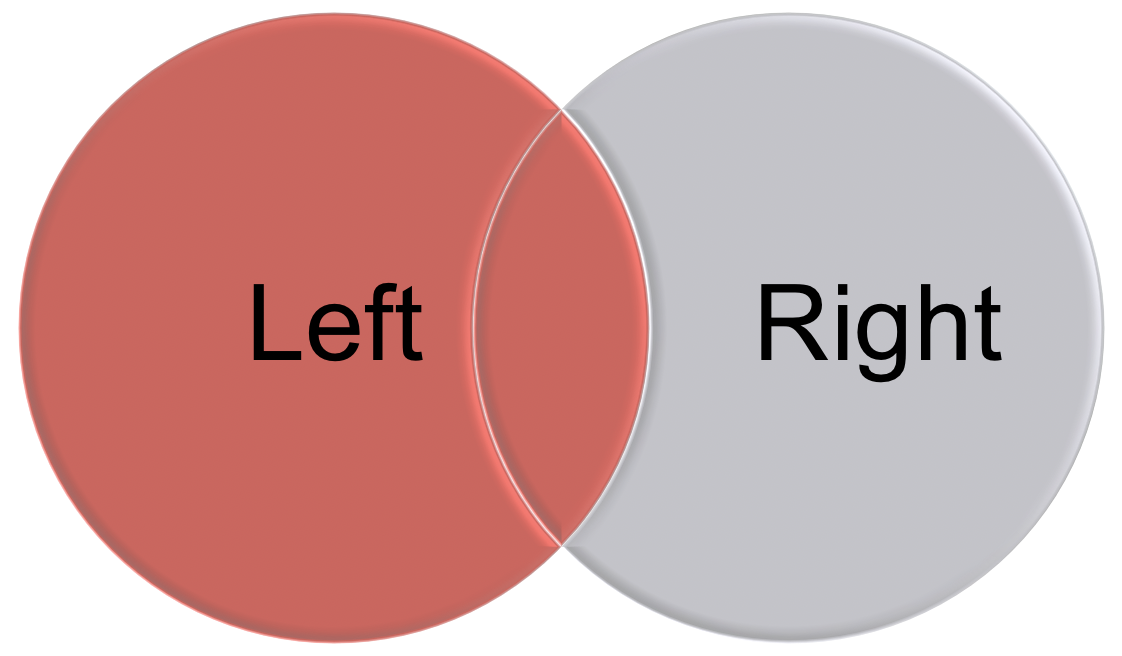

Figure 8.2: An illustration of left join and right join.
Different join functions control what happens to rows that exist in one table but not the other.
left_joinkeeps all the entries that are present in the left (first) table and excludes any that are only in the right table.right_joinkeeps all the entries that are present in the right table and excludes any that are only in the left table.inner_joinkeeps only the entries that are present in both tables.inner_joinis the only function that guarantees you won’t generate any missing entries.full_joinkeeps all of the entries in both tables, regardless of whether or not they appear in the other table.
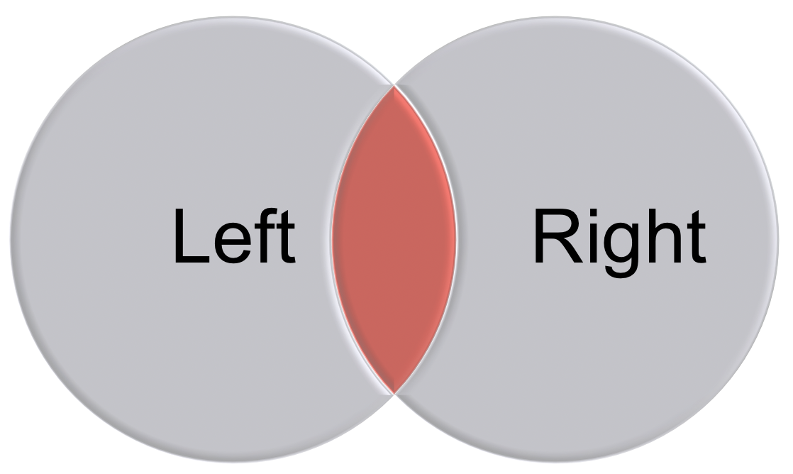
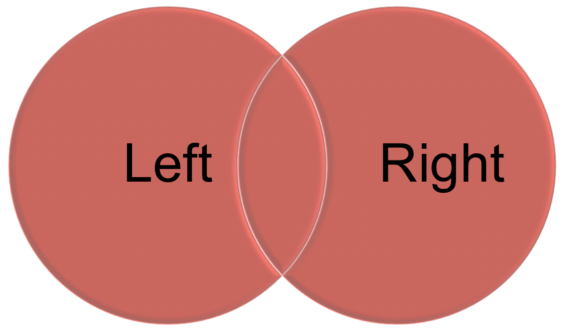
Figure 8.3: An illustration of inner join and full join.
The join functions are nicely illustrated in RStudio’s [Data wrangling cheatsheet][https://www.rstudio.com/wp-content/uploads/2015/02/data-wrangling-cheatsheet.pdf].
{r join, out.width = "80%", echo=FALSE, fig.align = "center", fig.cap="An illustration of the join functions in RStudio’s Data wrangling cheatsheet."} knitr::include_graphics("figures/dplyr-joins.png")
Toy examples with joins
set.seed(12345)
x <- data.frame(key= LETTERS[c(1:3, 5)],
                value1 = sample(1:10, 4),
                stringsAsFactors = FALSE)
y <- data.frame(key= LETTERS[c(1:4)],
                value2 = sample(1:10, 4),
                stringsAsFactors = FALSE)

x
##   key value1
## 1   A      3
## 2   B      8
## 3   C      2
## 4   E      5
y
##   key value2
## 1   A      8
## 2   B      2
## 3   C      6
## 4   D      3
# What's in both x and y?
inner_join(x, y, by = "key")
## key value1 value2
## 1 A 3 8
## 2 B 8 2
## 3 C 2 6# What's in X and bring with it the stuff that matches in Y
left_join(x, y, by = "key")
## key value1 value2
## 1 A 3 8
## 2 B 8 2
## 3 C 2 6
## 4 E 5 NA# What's in Y and bring with it the stuff that matches in Y
right_join(x, y, by = "key")
## key value1 value2
## 1 A 3 8
## 2 B 8 2
## 3 C 2 6
## 4 D NA 3# Give me everything!
full_join(x, y, by = "key")
## key value1 value2
## 1 A 3 8
## 2 B 8 2
## 3 C 2 6
## 4 E 5 NA
## 5 D NA 3# Want everything that doesn't match?
full_join(anti_join(x, y, by = "key"), anti_join(y, x, by = "key"), by= "key")
## key value1 value2
## 1 E 5 NA
## 2 D NA 3Practice with joins for real data
We first get the data named pop.county from the github R package slid. Note that there are four variables in this data: ID, County, State, population.
library(slid)
data(I.county)
dim(I.county)
## [1] 3104  328
data(pop.county)
dim(pop.county)
## [1] 3142    4
Now, we would like to join the two tables: I.county and pop.county using the left_join as follows:
I.county.w.pop <- left_join(I.county, pop.county, by = "ID") %>%
  dplyr::select(-c("County.y", "State.y"))
or we can:
8.8 Reshaping Data - Change the layout of a data set
Sometimes, we want to convert data from a wide format to a long format. Many functions in R expect data to be in a long format rather than a wide format. Programs like SPSS, however, often use wide-formatted data. There are two sets of methods that are explained below:
gather()andspread()from thetidyrpackage. This is a newer interface to thereshape2package.melt()anddcast()from thereshape2package.
Many other methods aren’t covered here since they are not as easy to use.
8.8.1 From wide to long
Below we would like to change the data I.state from wide format to long format.
Use gather(data, key, value, …)
data= the dataframe you want to morph from wide to longkey= the name of the new column that is levels of what is represented in the wide format as many columnsvalue= the name of the column that will contain the values…= columns to gather, or leave (use -column to gather all except that one)
The gather functions are nicely illustrated in RStudio’s [Data wrangling cheatsheet][https://rstudio.com/wp-content/uploads/2015/02/data-wrangling-cheatsheet.pdf] as shown in Figure 8.4.
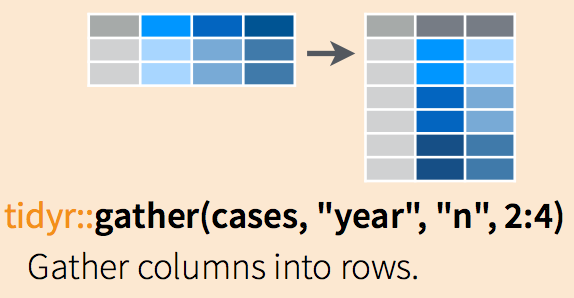
Figure 8.4: An illustration of gather function.
## [1] 49 326I.state.long <- gather(I.state.wide, DATE, Death,
X2020.12.11:X2020.01.22, factor_key = TRUE) %>%
arrange(State)
dim(I.state.long)## [1] 15925 3Use pivot_longer()
The function pivot_longer() is an updated approach to gather(), designed to be both simpler to use and to handle more use cases. It is recommended to use pivot_longer() for new code; gather() isn’t going away but is no longer under active development.
## [1] 49 326I.state.long <- I.state.wide %>%
pivot_longer(X2020.12.11:X2020.01.22,
names_to = "DATE", values_to = "Death")See more complicated examples from the introduction of ‘tidyr’ package.
8.8.2 From long to wide
Now let’s change the data back to the wide format, and we can use spread.
Use Use spread(data, key, value)
data= the dataframe you want to morph from long to widekey= the name of the column that contains the keyvalue= the name of the column contains the values
The spread functions are nicely illustrated in RStudio’s [Data wrangling cheatsheet][https://rstudio.com/wp-content/uploads/2015/02/data-wrangling-cheatsheet.pdf] as shown in Figure 8.5.
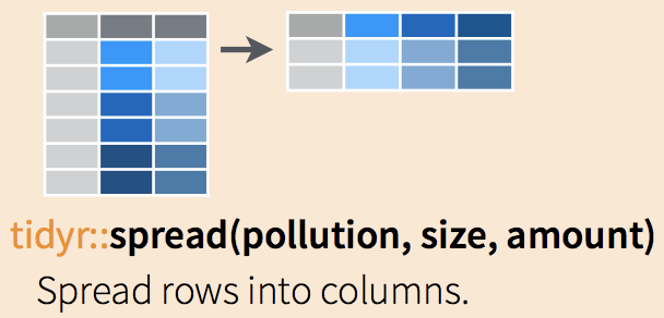
Figure 8.5: An illustration of spread function.
## [1] 49 326Use pivot_wider()
We can also use the function pivot_wider(), which “widens” data, increasing the number of columns and decreasing the number of rows. The inverse transformation is pivot_longer().
I.state.wide <- I.state.long %>%
pivot_wider(names_from = DATE, values_from = Death)
dim(I.state.wide)
## [1] 49 326See more complicated examples from the introduction of ‘tidyr’ package.
8.9 Exercises
We are going to explore the basic data manipulation verbs of dplyr using
nycflights13::flights. Install the R package nycflights13.
##  [1] "year"           "month"          "day"
##  [4] "dep_time"       "sched_dep_time" "dep_delay"
##  [7] "arr_time"       "sched_arr_time" "arr_delay"
## [10] "carrier"        "flight"         "tailnum"
## [13] "origin"         "dest"           "air_time"
## [16] "distance"       "hour"           "minute"
## [19] "time_hour"
Next, use ?flights to see more detailed information about this dataset.
- Select
dep_time,dep_delay,arr_time, andarr_delayfrom flights. - Find all flights on January 1st.
- Find all flights that departed in December.
- Find all flights that flew to Houston.
- Find all flights that were operated by United, American, or Delta.
- Sort flights to find the most delayed flights. Find the flights that left earliest.
- What does the following code provide?
delays <- flights %>%
  group_by(dest) %>%
  summarise(
    count = n(),
    dist = mean(distance, na.rm = TRUE),
    delay = mean(arr_delay, na.rm = TRUE)
)- What does the following code provide?