Chapter 2 R Introduction and Preliminaries
2.1 The R Environment and Language
R is an integrated suite of software facilities for data manipulation, calculation and graphical display.
The benefits of R for an introductory student
- R is free. R is open-source and runs on UNIX, Windows and Macintosh.
- R has an excellent built-in help system.
- R has excellent graphing capabilities.
- Students can easily migrate to the commercially supported S-Plus program if commercial software is desired.
- R’s language has a powerful, easy to learn syntax with many built-in statistical functions.
- The language is easy to extend with user-written functions.
- R is a computer programming language. For programmers it will feel more familiar than others and for new computer users, the next leap to programming will not be so large.
What is R lacking compared to other software solutions?
- There is no commercial support. (Although one can argue the international mailing list is even better)
- The command language is a programming language so students must learn to appreciate syntax issues etc.
R can be regarded as an implementation of the S language which was developed at Bell Laboratories by Rick Becker, John Chambers and Allan Wilks, and also forms the basis of the S-Plus systems.
R and SAS Comparison
R is in many ways comparable with SAS. The software is predominately syntax driven and relies on its user to known the R language (which in many ways resembles the S and UNIX programming languages). R is comparable in structure and conceptual arrangement to other syntax based software packages. Similarities and dissimilarities with other software packages will be pointed out to facilitate an easier transition into R.
Technically R is an expression language with a very simple syntax. Unlike SAS, it is case sensitive, so A and a are different symbols and would refer to different variables.
Commands are separated either by a semi-colon (“;”), or by a newline. Elementary commands can be grouped together into one compound expression by braces (“{” and “}”).
Comments can be put almost anywhere, starting with a hash-mark (“#”), everything to the end of the line is a comment.
If a command is not complete at the end of a line, R will give a different prompt, by default “+” on second and subsequent lines and continue to read input until the command is syntactically complete.
2.2 R and Statistics
Many people use R as a statistics system. We prefer to think of it as an environment within which many classical and modern statistical techniques have been implemented. A few of these are built into the base R environment, but many are supplied as packages. There are about 25 packages supplied with R (called “standard” and “recommended” packages) and many more are available through the CRAN family of Internet sites (via http://CRAN.R-project.org) and elsewhere. More details on packages are given later.
Most classical statistics and much of the latest methodology is available for use with R, but users may need to be prepared to do a little work to find it.
2.3 Installing R and RStudio
2.3.1 Obtaining R and installation
- Obtaining R
Sources, binaries, and documentation for R can be obtained via CRAN, the “Comprehensive R Archive Network” whose current members are listed at http://cran.r-project.org/mirrors.html.
- Installing R under Windows (via http://CRAN.R-project.org)
- The
bin/windowsdirectory of a CRAN site contains binaries for a base distribution and many add-on packages from CRAN to run on Windows 2000 or later on ix86 CPUs (including AMD64/EM64T chips and Windows x64). Your file system must allow long file names (as is likely except perhaps for some network-mounted systems). - Installation is straightforward. Just double-click on the icon and follow the instructions. You can uninstall R from the Control Panel or the (optional) R program group on the Start Menu.
- Installing R under Macintosh (via http://CRAN.R-project.org)
- Visit the Comprehensive R Archive Network (CRAN) and select a mirror site near you; a list of CRAN mirrors appears at the upper left of the CRAN home page. Click on the link Download R for Mac OS X, which appears near the top of the page; then click on R-X.X.X.pkg (or whatever is the current version of R), which assumes that you are using Mac OS X 10.9 (Mavericks) or higher. You will also find an older version of R if you have an older version of Mac OS X (10.6, Snow Leopard, or higher). Once it is downloaded, double-click on the R installer. You may take all of the defaults.
2.3.2 Installing RStudio
After you install R, you can install R Studio. Download and install RStudio at https://www.rstudio.com/products/rstudio/download/.
- Scroll down to “Installers for Supported Platforms” near the bottom of the page.
- Click on the download link corresponding to your computer’s operating system.
2.4 Starting R
RStudio is most easily used in an interactive manner. After installing R and RStudio on your computer, you’ll have two new programs (also called applications) you can open. We’ll always work in RStudio and not in the R application. Figure 2.1 below shows what icon you should be clicking on your computer.
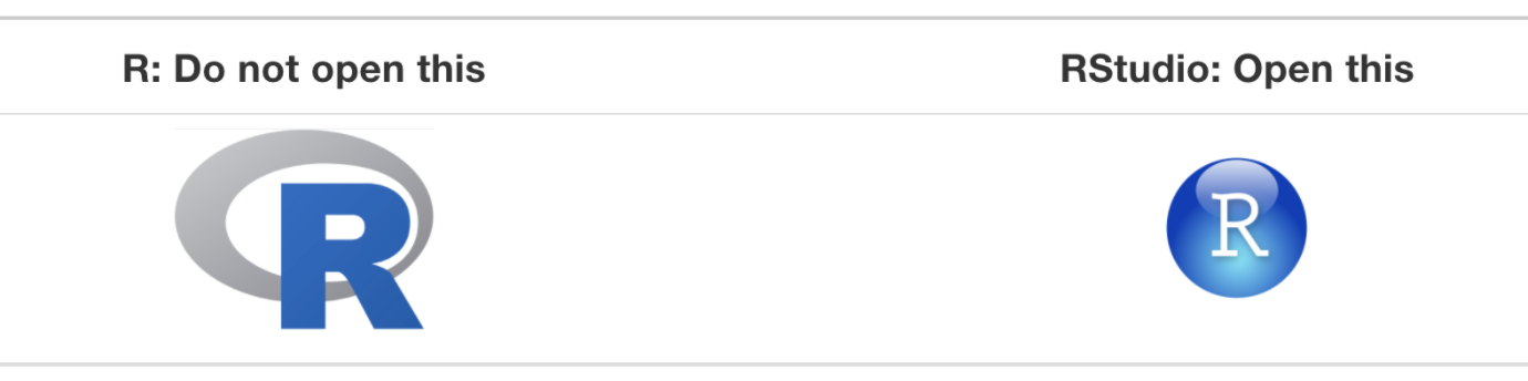
Figure 2.1: Icons of R versus RStudio on your computer.
After you open RStudio, you should see something similar to Figure 2.2 below.
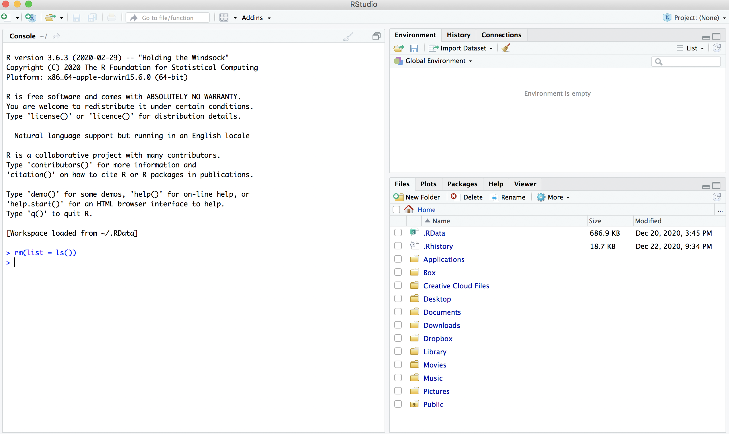
Figure 2.2: RStudio interface to R.
Note the three panels divide the screen: the console panel, the files panel, and the environment panel. Throughout this chapter, you’ll come to learn what purpose each of these panels serves.
Console: This is the place to write any code that needs to be run.
Environment: This lists what variables and objects (referred to in R) are currently available in your working environment. Within the environment window, there are also other tabs such as ‘history’, which shows a history of all code typed in the past. It also has a tab called ‘connection,’ which is meant for connecting to specific databases. This tab is not useful to a beginner.
Viewer: For lack of a better way to refer to the third pane, it is referred to here as ‘viewer.’ However, the third pane has several tabs nested within it. The “files” tab shows all the files and folders in your current directory, which the program points to right next to the home icon below the header for the pane. The “plots” tab shows and allows for the saving of any plot output. The “packages” tab shows all the packages that are currently installed. As you start using R-Studio, you will find the need to install many packages and R-Studio makes it easy to do so.
2.4.1 Description of three panels in user interface
- R Console window
- The R Environment contains the software’s libraries with all the available datasets, expansion packages and macros. As compared to SAS, the Log and Editor windows are consolidated into a single interface, the “R Console”.
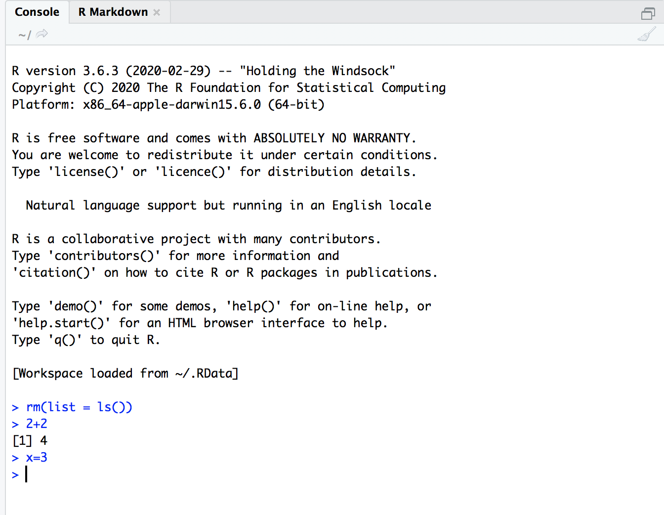
Figure 2.3: The R Console.
Note: The > is called the prompt. In what follows below it is not typed, but is used to indicate where you are to type if you follow the examples.
- The Console can be used like a calculator. Below are some examples:
- Results from these calculations can be stored in an object. The
<-is used to make the assignment and is read as “gets”.
- The objects are stored in R’s database. When you close R, you will be asked if you would like to save or delete them. This is kind of like the SAS WORK library, but R gives you a choice to save them. To see a listing of the objects, you can do either of the following:
- To delete an object, use
rm()and insert the object name in the parentheses.
- All objects created during an R session can be stored permanently in a file for use in future R sessions. At the end of each R session, you are given the opportunity to save all the currently available objects. If you indicate that you want to do this, the objects are written to a file called
.RDatain the current directory (“Save Workspace”), and the command lines used in the session are saved to a file called.Rhistory(“Save History”).
R Editor window – type your long R program here
Often, you will have a long list of commands that you would like to execute all at once, i.e., a program. Instead of typing all of the code line by line at the R Console, you could type it in the R Script Window. Select
File -> New File -> R scriptto create a new program. Below is what the editor looks like.To run the current line of the code (where the cursor is positioned) or some code highlighted, click “Run”.
To save your code as a program outside of R, select File -> Save and make sure to use an
.Rextension on the file name.
Error messages
R will provide intuitive error messages regarding the submitted syntax. Unlike in SAS these comments are printed right in the console.
R will provide intuitive error messages regarding the submitted syntax. Unlike in SAS these comments are printed right in the console.
2.4.2 R help
- To see a listing of all R functions which are “built in”, open the
Helpby selecting Help -> R Help from the main menu bar. Under Reference, select the link called Packages. All built-in R functions are stored in a package.
We have been using functions from the base and stats package. By selecting stats, you can scroll down to find help on the pnorm() function. Note the full syntax for pnorm() is
The q value corresponds to the 1.96 can be found by
pnorm(1.96)
## [1] 0.9750021
pnorm(q = 1.96)
## [1] 0.9750021
pnorm(q = 1.96, mean = 0, sd = 1)
## [1] 0.9750021
These produce the same results. The other entries in the function have default values set. For example, R assumes you want to work with the standard normal distribution by assigning mean=0 and sd=1 (standard deviation).
- If you know the exact name of the function, simply type
help(function name)at the R Console command prompt to bring up its help in a window inside of R. For example,
brings up Figure 2.4
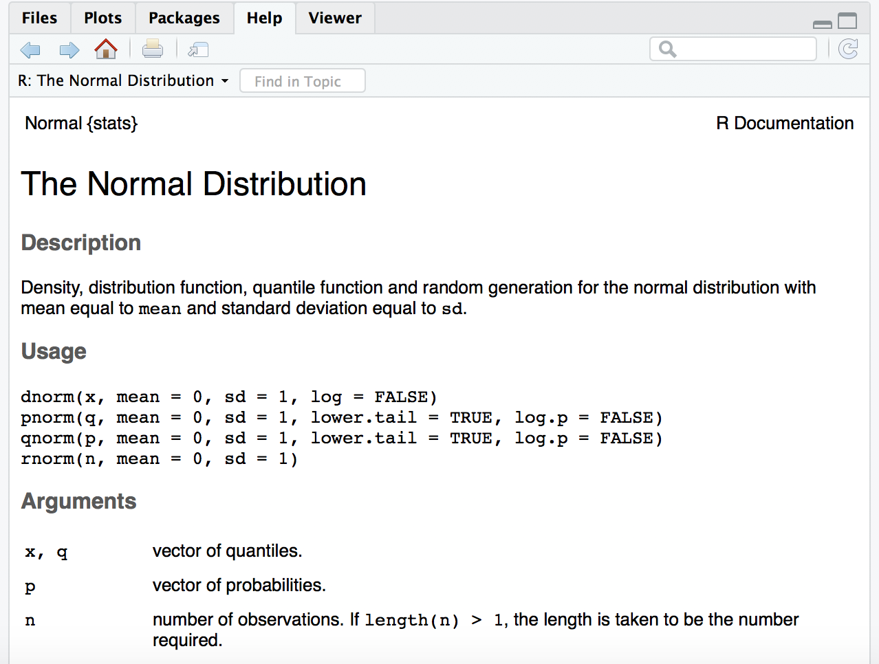
Figure 2.4: The R help for the R function pnorm().
An alternative is
For a feature specified by special characters, the argument must be enclosed in double or single quotes, making it a “character string”: This is also necessary for a few words with syntactic meaning including if and for functions.
- If you need to use a function but don’t know its exact name or are not sure of its existence. There is a very useful function called apropos(‘argument‘) that lists all functions that contain your argument as part of their names. Note that your argument must be put within either single or double quotation marks. For example, here is what I got when I looked for similar functions containing the string
table:
##  [1] ".S3_methods_table"   "[.table"
##  [3] "aperm.table"         "as.data.frame.table"
##  [5] "as.relistable"       "as.table"
##  [7] "as.table.default"    "ftable"
##  [9] "is.relistable"       "is.table"
## [11] "margin.table"        "model.tables"
## [13] "pairwise.table"      "print.summary.table"
## [15] "print.table"         "prop.table"
## [17] "r2dtable"            "read.ftable"
## [19] "read.table"          "summary.table"
## [21] "table"               "write.ftable"
## [23] "write.table"         "xyTable"
Note that the argument is a string, so it does not need to be an actual word or name of a function. For example, apropos('tabl') will return the same results. Try it!
- There may be other times when you want to learn about all functions involving a certain term, but searching for R-related pages on that term returns too many irrelevant results. This term may not even be an R function or command, making the Google search all the more difficult, even with good searching techniques. In these situations, use the
help.search(‘argument‘)function. (Again, you need to put your arguments around single or double quotation marks.) This will return all functions with your argument in the help page title or as an alias.
For example, I wanted to know about using PDF files in R. I ran help.search(‘pdf’) in R and got the following results.
2.4.3 Packages
This is a very important topic in R. In SAS and SPSS installations, you usually have everything you have paid for installed at once. R is much more modular. The main installation will install R and a popular set of add‐ons called libraries. Hundreds of other libraries are available to install separately from the Comprehensive R Archive Network, (CRAN).
Right under the “viewer” tab, the icon for “setting” allows for changing the working directory or copying and moving files. The tab for “packages,” shows all the packages that are installed and available. Clicking on the checkbox next to the name of the package loads the package for use using the following command, which will appear in the console pane of the interface.
Clicking on the name of the package (under the package tab on the lower right pane) itself brings up the description of what the package does. This is one of the benefits of using R-Studio as opposed to R, which makes it easy to look up all the packages available and what each does. Although the description and examples for packages are sometimes not explicit enough, it is nevertheless a useful starting point for many tasks. The viewer pane tab also makes it easy to install and update packages right from the lower right panel of the user interface.
If you want to use functions in other packages, you may need to install and then load the package into R. Packages if they have already been downloaded from a CRAN mirror site can be loaded using this procedure. If the package has not been downloaded, it can be installed using the
Install package(Package name)option. Also, an installed package can be loaded by specifyinglibrary (name of package).For example, we will be using the
ggplot2package later for data visualization.- While in the R console, select Tools -> Install Packages from the main menu.
- A number of locations around the world will come up. Insert the
ggplot2package and selectInstall.
- The package will now be installed onto your computer. This only needs to be done once on your computer. To load the package into your current R session, type
library(ggplot2)at the R Console prompt. This needs to be done only once in an R session. If you close R and reopen, you will need to use thelibrary()function again. - If the package contains example data sets, you can load them with the data command. Enter
data()to see what is available and thendata(mydata)to load one named, for example,mydata.
Clicking on the link to the package name from within the “packages” tab in the viewer pane provides an overview of what the package does. Here it is useful to spend some time understanding how to use a package. Clicking on the link provides details on its documentation. Next to the package is the package title, which states, “Create Elegant Data Visualisations Using the Grammar of Graphics.” Thus, ggplot2 is a package that makes elegant data visualizations. Clicking on the package link provides an alphabetized list of all that the package does, such as a function called aes that helps construct aesthetic mappings. Another function called borders helps to create a layer of map borders.
Clicking on the link aes provides an explanation for what the function does and the way (syntax) it is used. Understanding the structure of this description helps us understand how to use packages. The description of the function within the package has several parts to it as follows:
Description: Aesthetic mappings describe how variables in the data are mapped to visual properties (aesthetics) of geoms. Aesthetic mappings can be set in ggplot() and in individual layers.
Usage: The second aspect of the description of the function refers to its usages.
Arguments: The third part of the structure of a function is referred to as arguments. This describes the objects or variables that this function will operate on.
Example: Typically, any description of what a function does is accompanied by an example of how to use it.
Thus, understanding how to install a package, the functions it is capable of, along with the examples its description provides makes R very versatile for the user. In the next chapter, we will learn how to use R and its basic functions.
2.4.4 Creating a project and setting working directory
Before launching into creating a dataset, it is important to understand how R handles data from a filing and directory perspective. Before creating a dataset, R starts with the creation of a ‘new project.’ A project name is a name given to a folder that will hold everything associated with a specific project such as data, history of commands used, objects (In R, a variable and/or data are stored as “objects”), or variables are created.
Along with creating a new project name, it is important to understand the concept of the working directory as R will look for variables and objects or any other files that are being called in the working directory. A simple way to check on the current working directory is to type the command getwd() into the command console. If it is not the intended directory you want to use, the simplest way to change it is by using the “viewer” pane and clicking on the tab that says ‘more.’ Ensuring that your working directory is where you want your files and objects created to be stored is important, especially to a beginner.
You may now create a new project by opening R-Studio, clicking on the file, and then ‘new project.’ As shown in Figure 2.5 that opens asks if you would like to open the project in an existing directory, a new one, or simply version control. The existing directory is the directory that is currently the working directory. You may either choose an existing directory or a new one. However, if you choose a new one, you need to make sure that it is selected as the working directory as shown earlier. You may name your project as ‘Learning R.’
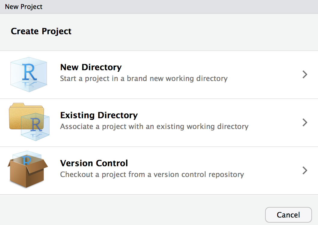
Figure 2.5: Interface for creating a project in R.
Once the project is created, you will see a .proj file under the files section in the viewer pane, as shown in Figure 2.6. As the figure shows, a new project called ‘Learning R.rproj’ has been created in the directory ~/STAT 480/Learning R. Any work done will now be stored in this directory (by setting it as the working directory) and in this project as long as it is saved when you exit.
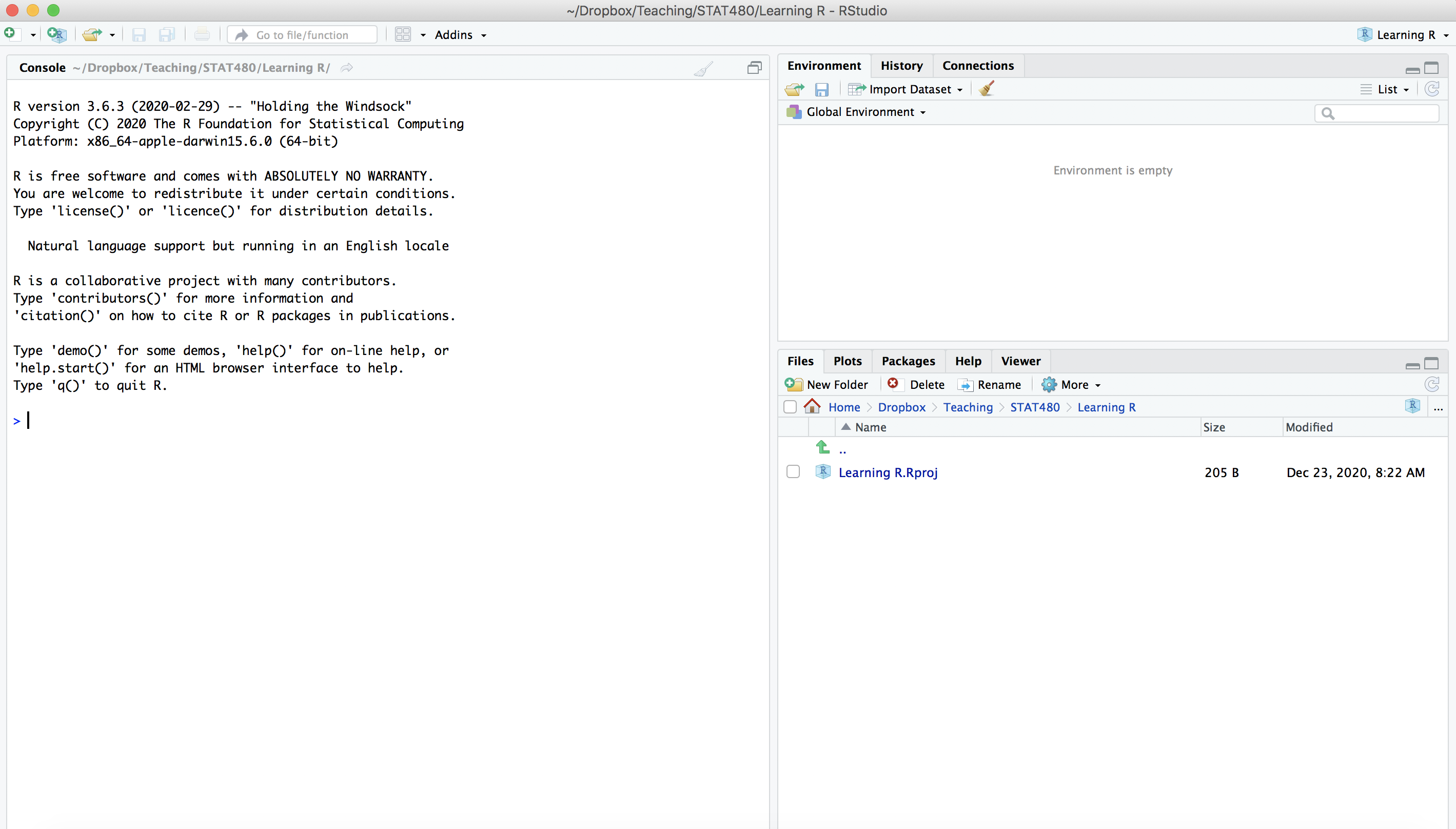
Figure 2.6: Directory with new project.
2.5 Exercises
- Use R to do the following
- Assign the value of 39 to
x.
- Assign the value of 22 to
y. - Make
zthe value ofx - y. - Display the value of
zin the console
You can use R for magic tricks: Pick any number. Double it, and then add 12 to the result. Divide by 2, and then subtract your original number. Did you end up with 6.0?
Use R to calculate the following:
- \(31 \times (78-20)^2\)
- \(697/41\)
- \(\sqrt{123}\)
- Download a dataset from Principles of Econometrics and save it in your local folder. Install the package
readxland read in the excel dataset you saved.