Chapter 5 Export/Import Data
In this chapter, you’ll learn how to read plain-text rectangular files into R, and how to export data from R to txt, csv, and R data file formats.
5.1 Data Export
Using function cat()
The function cat is useful for producing output in user-defined functions.
## Good morning!Using function print()
The function print prints its argument. It is a generic function which means that new printing methods can be easily added for new classes.
## [1] "Good morning!"Write a matrix or data frame to file
The commonest task is to write a matrix or data frame to file as a rectangular grid of numbers, possibly with row and column labels. This can be done by the functions write.table and write.
- Command to copy and paste from R into Excel or other programs. It writes the data of an R data frame object into the clipboard from where it can be pasted into other applications.
age <- 18:29
height <- c(76.1, 77, 78.1, 78.2, 78.8, 79.7, 79.9, 81.1, 81.2,
            81.8, 82.8, 83.5)
village <- data.frame(age = age,height = height)

# Write village into clipboard
write.table(village, "clipboard", sep = "\t", col.names = NA,
            quote = F)
Remark:
The argument quote is a logical value (
TRUEorFALSE) or a numeric vector. IfTRUE, any character or factor columns will be surrounded by double quotes. IfFALSE, nothing is quoted.The argument
col.names= NAmakes sure that the titles align with columns when row/index names are exported (default).
- Write data frame to a tab-delimited text file.
write.delim(village, file = "village.txt")
# provides same results as read.delim
write.table(village, file = "village.txt", sep = "\t")- Write data to csv files:
- Write matrix data to a file.
Remark: write.table() is the multipurpose work-horse function in base R for exporting data. The functions write.csv() and write.delim() are special cases of write.table() in which the defaults have been adjusted for efficiency.
5.1.1 .RData files
The best way to store objects from R is with .RData files. .RData files are specific to R and can store as many objects as you’d like within a single file.
** The save() function
age <- 18:29
height <- c(76.1, 77, 78.1, 78.2, 78.8, 79.7, 79.9, 81.1, 81.2,
            81.8, 82.8, 83.5)
village <- data.frame(age = age, height = height)

# Save the object as a new .RData file
save(village, file = "data/village.rda")
To save selected objects into one .RData file, use the save() function. When you run the save() function with specific objects as arguments, (like save(a, b, c, file = "myobjects.RData") all of those objects will be saved in a single file called myobjects.RData. For example, let’s create a few objects corresponding to a study.
5.2 Data Import
5.2.1 The load() function
To load an .RData file, that is, to import all of the objects contained in the .RData file into your current workspace, use the load() function. For example, to load the three specific objects that I saved earlier (study1.df, score.by.sex) in study1.rda, I’d run the following:
To load all of the objects in the workspace that we have saved to the data folder in a working directory named projectnew.rda, we can run the following:
5.2.2 The read.table() function
Large data objects will usually be read as values from external files rather than entered during an R session at the keyboard. R input facilities are simple, and their requirements are fairly strict and even rather inflexible.
If variables are to be held mainly in data frames, as we strongly suggest they should be, an entire data frame can be read directly with the read.table() function. There is also a more primitive input function, scan(), that can be called directly. For more details on importing data into R and also exporting data, see the R Data Import/Export manual.
To read an entire data frame directly, the external file will typically have a special form.
- The first line of the file should have a name for each variable in the data frame.
- Each additional line of the file has its first item, a row label, and the values for each variable.
By default, numeric items (except row labels) are read as numeric variables and non-numeric variables, such as name and gender in the above example, as factors.
The function read.table() can then be used to read the data frame directly. For the file, scores_names.txt, you might want to omit, including the row labels, directly and use the default labels.
In this case, the file may omit the row label column as in the following.
where the header=TRUE option specifies that the first line is a line of headings, and hence, by implication from the form of the file, that no explicit row labels are given. This can be changed if necessary.
scores <- read.table("scores_names.txt",
                     colClasses = c("character", "character",
                                    "integer", "integer"),
                     header = TRUE)
> scores[['gender']]
If the values are separated by commas or another “delimiter,” we have to specify the delaminating character(s). For example, look at the file reading.txt on the Blackboard folder.
reading <- read.table("reading.txt", sep = ",")

# names() is to get or set the names of an object.
names(reading) = c("Name", "Week1", "Week2", "Week3",
                   "Week4", "Week5")
print(reading)
If sep = "" (the default for read.table) the separator is ‘white space’, that is one or more spaces, tabs, newlines or carriage returns.
5.2.3 The scan() function
In fact read.table() uses scan() to read the file, and then process the results of scan. It is very convenient, but sometimes it is better to use scan() directly.
- The function
scan()at its simplest can do the same as c. It saves you having to type the commas though:
Note that we start typing the numbers in z. If we hit the return key once we continue on a new row, if we hit it twice in a row, the scan stops. This can be fairly convenient when entering in a few data points (10-40 say).
- Using scan with a file
The file ReadWithScan.txt in your drive has contents
1 2 3
4
Then, the command
will read the contents into your R session.
Now suppose you had some formatting between the numbers you want to get rid of for example this is now your file ReadWithScan.txt
1, 2, 3,
4
then
works.
- The function scan has many arguments in common with
read.table. One additional argument is what, which specifies a list of modes of variables to be read from the file. If the list is named, the names are used for the components of the returned list. Modes can be numeric, character or complex, and are usually specified by an example, e.g., 0 or "".
Suppose the data vectors are of equal length and are to be read in parallel. Further, suppose that there are three vectors, the first of mode character and the remaining two of mode numeric, and the file is ‘input.dat’. The first step is to use scan() to read in the three vectors as a list, as follows:
Read 3 records:
[[1]]
[1] "A" "B" "C"

[[2]]
[1] 2 2 6

[[3]]
[1] 1 3 7
The second argument is a dummy list structure that establishes the mode of the three vectors to be read. The result, held in inp, is a list whose components are the three vectors read in. To separate the data items into three separate vectors, use assignments like
More conveniently, the dummy list can have named components, in which case the names can be used to access the vectors read in. For example,
There are more elaborate input facilities available and these are detailed in the manuals.
5.2.4 The read.csv() function
Alternatively, you may have data from a spreadsheet. The simplest way to enter this into R is through a file format. Typically, this is a CSV format (comma-separated values). First, save the data from the spreadsheet as a CSV file say data.csv. Then the R command read.csv will read it in as follows
CSV file can be comma delimited or tab or any other delimiter specified by parameter sep =. If the parameter header = is TRUE, then the first row will be treated as the row names.
read.csv(file, header = FALSE, sep = ",", quote = "\"", dec = ".",
         fill = TRUE, comment.char = "", ...)
read.csv2(file, header = TRUE, sep = ";", quote = "\"", dec = ",",
fill = TRUE, comment.char = "", ...) file: file nameheader: 1st line as header or not, logicalsep: field separatorquote: quoting characters …
The difference between read.csv and read.csv2 is the default field seperator, as “,” and “;” respectively. Following is a csv file example:
t1	t2	t3	t4	t5	t6	t7	t8
r1	1	0	1	0	0	1	0	2
r2	1	2	2	1	2	1	2	1
r3	0	0	0	2	1	1	0	1
r4	0	0	1	1	2	0	0	0
r5	0	2	1	1	1	0	0	0
r6	2	2	0	1	1	1	0	0
r7	2	2	0	1	1	1	0	1
r8	0	2	1	0	1	1	2	0
r9	1	0	1	2	0	1	0	1
r10	1	0	2	1	2	2	1	0
r11	1	0	0	0	1	2	1	2
r12	1	2	0	0	0	1	2	1
r13	2	0	0	1	0	2	1	0
r14	0	2	0	2	1	2	0	2
r15	0	0	0	2	0	2	2	1
r16	0	0	0	1	2	0	1	0
r17	2	1	0	1	2	0	1	0
r18	1	1	0	0	1	0	1	2
r19	0	1	1	1	1	0	0	1
r20 0 0 2 1 1 0 0 15.2.5 Import an Excel file into R
You can import an excel file using the readxl package. To start, here is a template that you can use to import an Excel file into R:
If you want to import a specific sheet within the Excel file, you may use this template:
If you want to set a three column excel sheet to contain the data as dates in the first column, characters in the second, and numeric values in the third, you would need the following lines of code:
5.2.6 Accessing built-in datasets
Around 100 datasets are supplied with R (in package datasets), and others are available in packages (including the recommended packages supplied with R). To see the list of datasets currently available use data().
As from R version 2.0.0 all the datasets supplied with R are available directly by name.
However, many packages still use the earlier convention in which data was also used to load datasets into R, for example,
and this can still be used with the standard packages. In most cases this will load an R object of the same name. However, in a few cases it loads several objects, so see the on-line help for the object to see what to expect.
Loading data from other R packages
To access data from a particular package, use the package argument, for example,
Figure 5.1 shows a subset oof supported file formats.
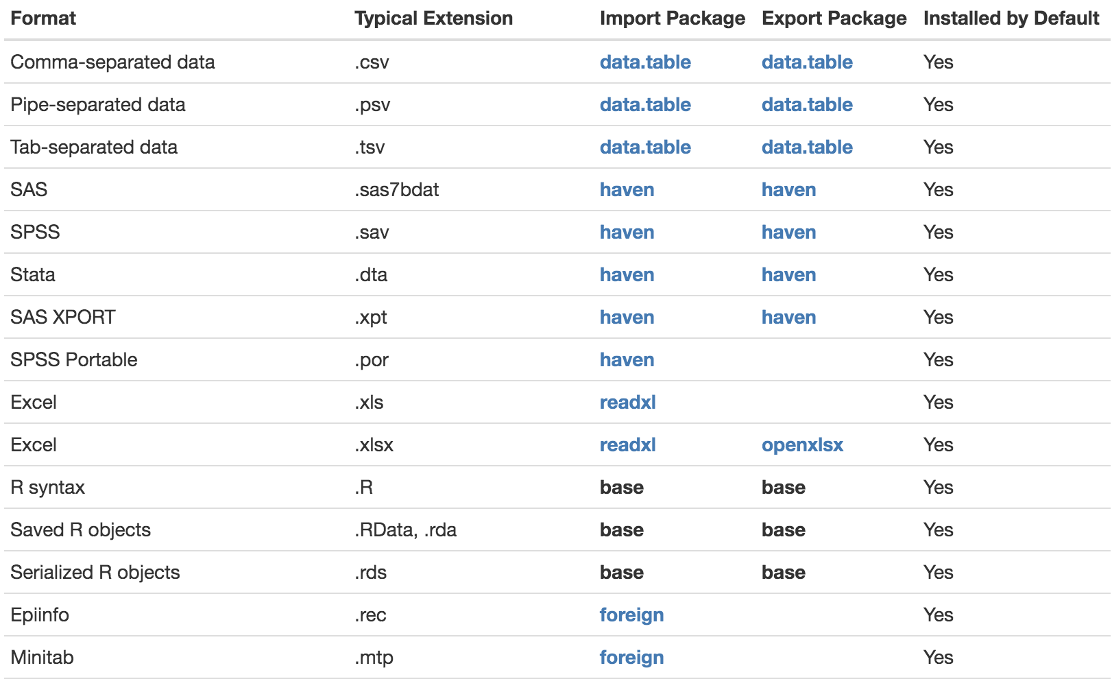
Figure 5.1: A non-inclusive list of supported file formats.