Chapter 7 R Markdown
R Markdown is a convenient feature of RStudio that allows you to keep your R code, results, and commentary in one file.
R Markdown (.Rmd) is an authoring format that enables easy creation of dynamic documents, presentations, and reports from R. It combines the core syntax of markdown (an easy to write plain text format) with embedded R code chunks that are run so their output can be included in the final document. R Markdown documents are fully reproducible (they can be automatically regenerated whenever underlying R code or data changes).” – RStudio documentation.
R Markdown has 3 main purposes:
- To communicate results to people who are more interested in your conclusions than how your reached them;
- To collaborate with other statisticians who are interested in both your code and your results;
- To function somewhat like a lab notebook: you can include your code and the reasoning behind it so you can easily understand and share what you did.
R Markdown documents are fully reproducible and support dozens of static and dynamic output formats. Three of the most common formats are:
- HTML
- Word documents
If you prefer a video introduction to R Markdown, we recommend that you check out the website https://rmarkdown.rstudio.com, and watch the videos in the “Get Started” section, which cover the basics of R Markdown.
In this chapter, we provide a very basic introduction of R Markdow. RStudio has created an R Markdown cheat sheet, which are freely available at https://www.rstudio.com/resources/cheatsheets/. More details of R Markdown can be found from https://bookdown.org/yihui/rmarkdown/.
Installation
Like the rest of R, R Markdown is free and open source. You can install the R Markdown package from CRAN with:
To produce PDF documents, you will also need to install * MiKTex: https://miktex.org/download (Windows users) * MacTeX: https://www.tug.org/mactex/mactex-download.html (Mac users)
7.1 Getting Started with R Markdown
Open RStudio. At the top of the screen, click on “File”, “New File”, “R Markdown”. This will bring up a dialog box that looks something like the image on the right (Mac version).
You can enter a title for your document and enter your name in the “Author” field. Next, you need to choose your output format. HTML is the default, though you can also choose PDF or a Word document. After you click OK, the R Markdown workspace will be generated.
7.2 Formatting Your Document
At the top of a default R Markdown document, you will see something that looks like this:
---
title: "Untitled"
author: "Your Name"
date: "12/12/2020"
output: pdf_document
---
This is called the YAML header. We can include more options to further customize our document.
YAML Header Options
- The
geometryoption lets you change the margins of your document.
- The
fontsizeoption changes the font size in your document.
- Specifying
pagenumber: TRUEadds page numbers to your document.
- If you would like to use the report format that generates a convenient title page, include
documentclass: report.
You may find the report document class useful when creating your report. The report format automatically makes a title page for your document. You will need to format your headers like this: ##Header. Otherwise, your headers will be preceded by “Chapter 1” and so on.
This is how to use the report template in your document:
---
title: "Untitled"
author: "Your Name"
date: "12/12/2020"
output: pdf_document
pagenumber: TRUE
geometry: margin=1in
fontsize: 12pt
documentclass: report
---
7.3 Text Formatting
In R Markdown, you can type regular text without having to make everything a comment. Usually, LaTeX commands will work.
- To make a new line, put 2 spaces at the end of the line before and then start the new line.
- To italicize text, use italics or italics.
- To make text bold, use bold or bold.
- To make a superscript, use
x^2^for normal text or \(x^2\) to make a subscript for an equation.
- To make a subscript, use
x~0~for normal text or \(x_0\) to make a subscript for an equation.
7.4 Greek Alphabet
Many statistical expressions use the Greek alphabet, so it is good to know how to use Greek letters in R Markdown.
- This is alpha: \(\alpha\)
- This is beta: \(\beta\)
- This is epsilon: \(\epsilon\)
- This is the equation for the univariate linear regression model: \(y_i = \beta_0 + \beta_1x_i + \epsilon_i\).
- This is the prediction equation for y based on \(x_i\): \(\hat{y_i} = \hat{\beta_0} + \hat{\beta_1}x_i\).
7.5 R code chunks and inline R code
There are a lot of things you can do in a code chunk: you can produce text output, tables, or graphics. You have fine control over all these output via chunk options, which can be provided inside the curly braces. For example, you can choose hide text output via the chunk option results = 'hide', or set the figure height to 4 inches via fig.height = 4. Chunk options are separated by commas, e.g.,
{r, chunk-label, results='hide', fig.height=4}There are a large number of chunk options in knitr documented at https://yihui.name/knitr/options. We list a subset of them below:
eval: Whether to evaluate a code chunk.echo: Whether to echo the source code in the output document (someone may not prefer reading your smart source code but only results).results: When set to'hide', text output will be hidden; when set to'asis', text output is written “as-is,”.warning,message, anderror: Whether to show warnings, messages, and errors in the output document. Note that if you seterror = FALSE,rmarkdown::render()will halt on error in a code chunk, and the error will be displayed in the R console. Similarly, whenwarning = FALSEormessage = FALSE, these messages will be shown in the R console.
Rendering Output
There are two ways to render an R Markdown document into its final output format. If you are using RStudio, then the “Knit” button (Ctrl+Shift+K) will render the document and display a preview of it.
If you are not using RStudio then you simply need to call the rmarkdown::render function, for example:
7.6 Including Plots and Adding Captions
You can embed plots and add captions.
Figure 7.1 shows a plot of the built-in trees dataset.
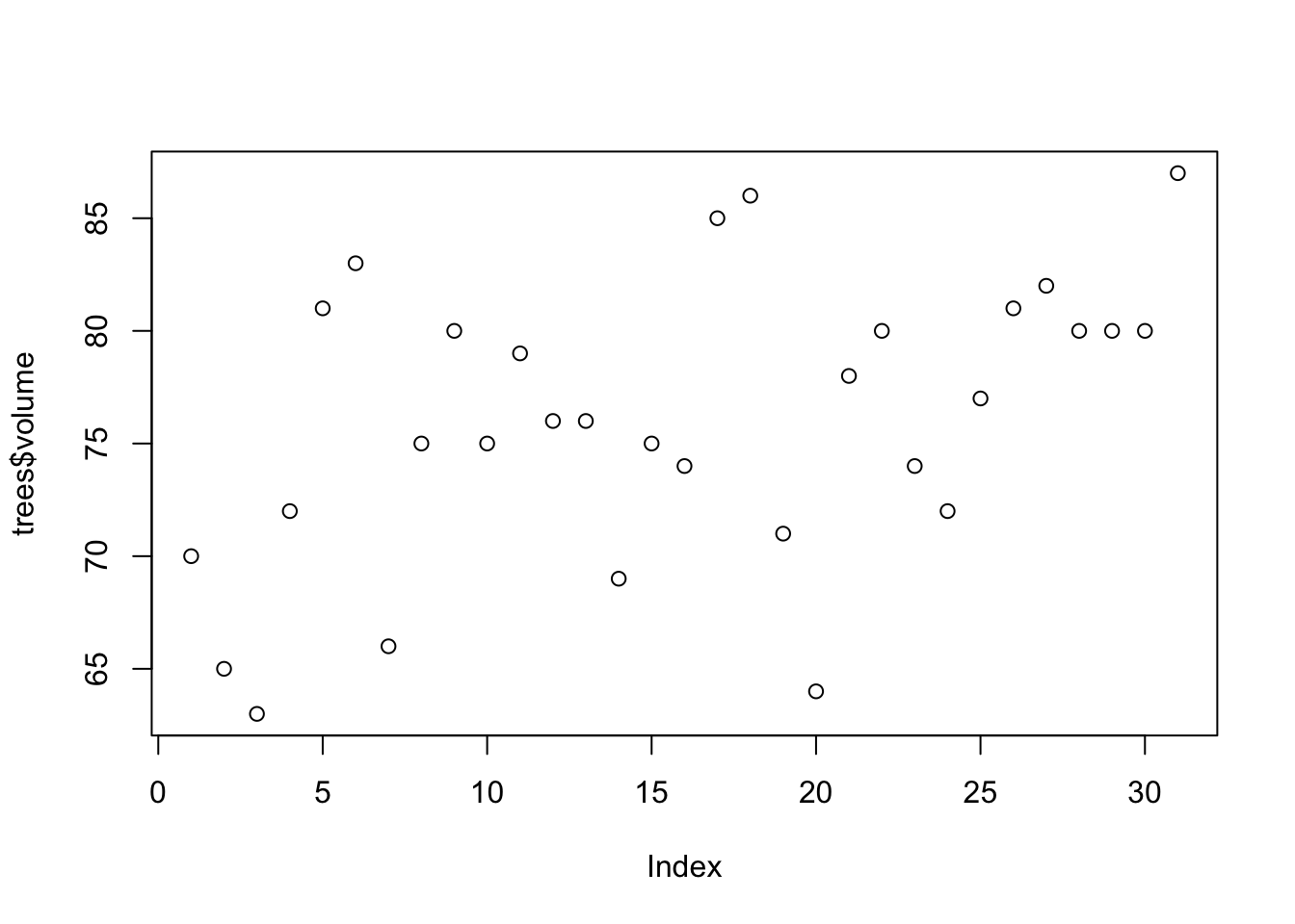
Figure 7.1: An example of a simple plot.
7.7 Modifying Figures
What if we would like to change the size of the plot?
The fig.height option lets us specify how tall we want the plot to be, the fig.width option lets us specify how wide we want the plot to be, and the fig.align option lets us specify whether we want the plot to be left-aligned, centered, or right-aligned. An example is shown in Figure 7.2.
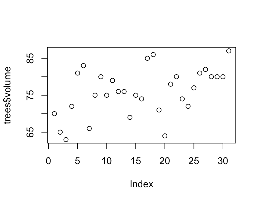
Figure 7.2: A smaller version of the plot.
7.8 Displaying Data with kable
You can make nice-looking tables that are not in plain text with kable. Compare the kable to the plain-text version of the data.
| temperature | pressure |
|---|---|
| 0 | 0.0002 |
| 20 | 0.0012 |
| 40 | 0.0060 |
| 60 | 0.0300 |
| 80 | 0.0900 |
| 100 | 0.2700 |
| 120 | 0.7500 |
| 140 | 1.8500 |
| 160 | 4.2000 |
| 180 | 8.8000 |
| 200 | 17.3000 |
| 220 | 32.1000 |
| 240 | 57.0000 |
| 260 | 96.0000 |
| 280 | 157.0000 |
| 300 | 247.0000 |
| 320 | 376.0000 |
| 340 | 558.0000 |
| 360 | 806.0000 |
##    temperature pressure
## 1            0   0.0002
## 2           20   0.0012
## 3           40   0.0060
## 4           60   0.0300
## 5           80   0.0900
## 6          100   0.2700
## 7          120   0.7500
## 8          140   1.8500
## 9          160   4.2000
## 10         180   8.8000
## 11         200  17.3000
## 12         220  32.1000
## 13         240  57.0000
## 14         260  96.0000
## 15         280 157.0000
## 16         300 247.0000
## 17         320 376.0000
## 18         340 558.0000
## 19         360 806.0000
7.9 Compiling R Markdown Documents
When you want to see what your compiled R Markdown document looks like, click on the ball of yarn at the top of the workspace to “knit” or compile the document. You can see the progress as your document is knitted in the “R Markdown” tab in the Console window at the bottom of the screen. If there is a problem, the knitting process will stop and an error message will appear in the R Markdown Console window. The error message tells you the line where the first error occurred so you can go back and fix it. Once the error is fixed, try knitting the document again. The process continues until the document is error-free and the output file can be produced.